
I saw a circuit simulator video on a Brazilian channel. A PT100 wired to a transmitter, 0–10 V coming out the other side, all shown on screen. One thought: if our GO Modular IO could do that, we could show people how the product behaves before they have ever touched one. Control is the job of the Senbrix PLC; the modules handle its IO.
It doubles as pre-launch promotion, and as a way to try wiring and programs without the hardware.
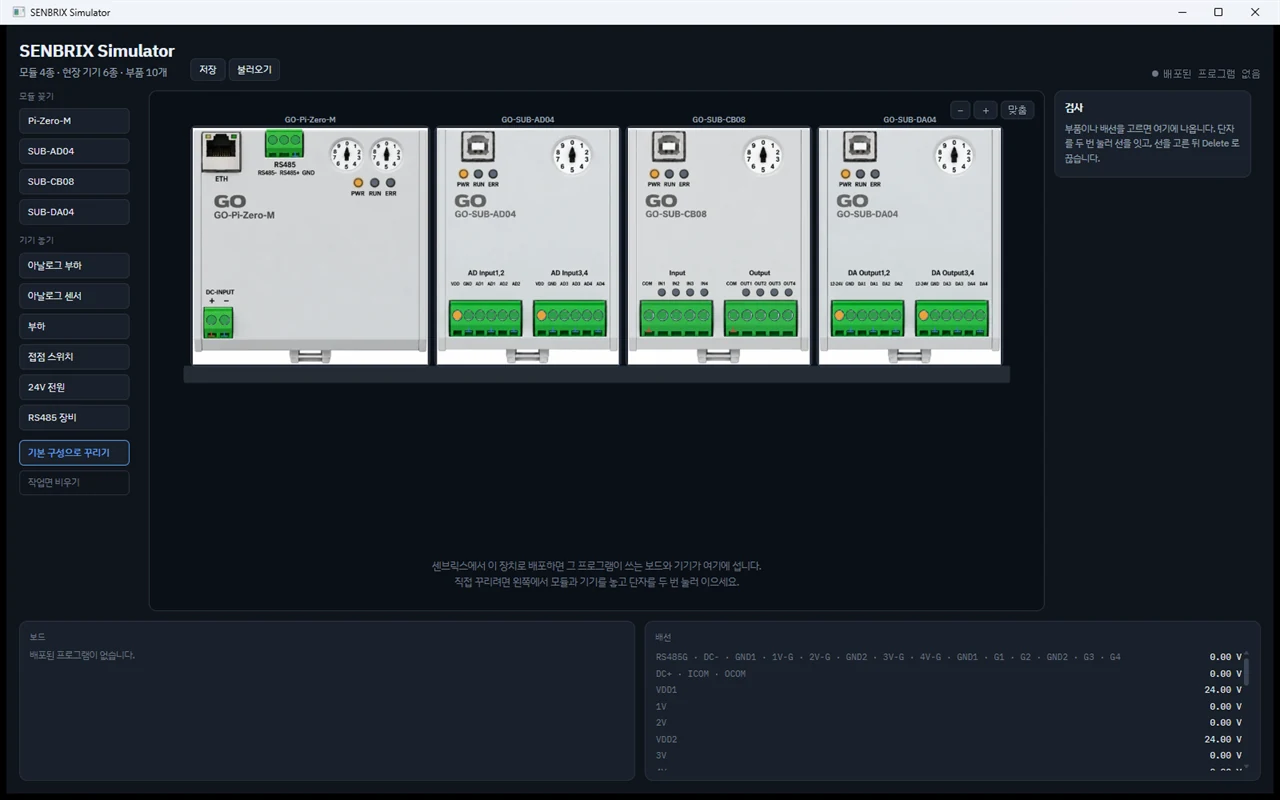
We named it the SENBRIX Simulator. It is what the Senbrix editor deploys to, so it takes that name.
Instead of imitating the controller, we put the whole thing inside
The first idea was a simulator running in the browser. Draw the modules, add a few IF/THEN rules to imitate the behavior. We actually started that way and it worked fine.
The problem is that it is not the real thing. The rules on screen are an imitation we wrote; what runs on the real controller is the program the editor compiled. Once the two start drifting apart, the simulator cannot be trusted. Nothing is more useless than “it worked in the sim”.
So we changed direction.
The compiled program the editor deployed     ← real
The deployed board drivers                   ← real
  The path to the boards (a CAN wire on HW)  ← only this is virtual
The simulator bench (sensors, switches, loads, wiring)
The controller runtime was put inside the simulator whole. The board drivers are the ones the real hardware uses. Only one place changed: where the CAN wire sits on hardware, a virtual bus is plugged in.
So the deployed program does not know it is inside a simulator. The scan period and the way boards exchange frames are the same as on hardware. With nothing imitated, there is nowhere to drift.
Deploy, and the screen wires itself
This is where it gets interesting.
When you create a project in the editor, the project already knows which boards it uses. It is all written in the deployment. So the simulator reads that and lays out the rail.
Open the editor’s connection window and SenbrixSim appears in the list next to the Raspberry Pis. Press deploy exactly as you would for hardware. Then
- The modules the program uses appear on the rail. Two IO modules in the program means two on the rail
- A device is placed on every channel and the wiring is drawn
- Input channels get something that produces a signal (a switch, a sensor); output channels get something that shows a result (a lamp, a meter)
Only the channels the program actually uses are furnished. Channels touched directly in code and channels bound through addresses are told apart, so no device is hung on a terminal nothing uses.
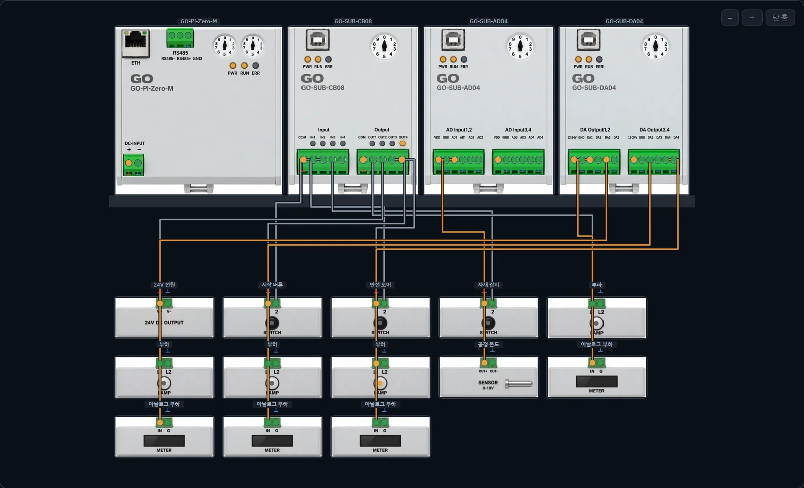
The bench right after a deploy. Switches on three contact inputs, lamps on the contact outputs, a sensor on the analog input and meters on the analog outputs, all wired. Power and ground are not drawn as wires — the reason is below.
The names from the interview come along
When the editor creates a project it asks what you are building. The answers contain names — start button, safety door, process temperature.
Those names reach the simulator.
| Board terminal | Address | Name |
|---|---|---|
| CB08 IN0 | P0 | Start button |
| CB08 IN1 | P1 | Safety door |
| CB08 IN2 | P2 | Material detect |
| AD04 AI0 | D0 | Process temperature (℃) |
The switch on screen is labeled “Start button”, not “contact switch”. A channel answered in ℃ gets a sensor that reports in ℃. When you are explaining the wiring, that difference matters.
Commons are not drawn
At first every power, ground and COM was drawn as a wire. Honest, but the screen became unusable. Commons filled the bench and the signal wires were buried between them; you could not read what went where.
That is why real wiring diagrams mark ground with a symbol only.
So every terminal got a common rail. Terminals on the same rail count as connected without a wire; a small ground symbol is printed under the terminal.
And the rail is the user’s choice. That turned out to matter more than expected.
A switch does not turn on just because it closes
Think of a dry contact switch. Tie one leg to 24 V and it passes 24 V when closed. Tie it to 0 V and closing it passes nothing.
Where one leg is tied is what flows. And that is also the spot most often wired wrong in the field.
So the simulator behaves that way. A switch passes whatever voltage is actually present on its supply side. The inspector shows it like this.
Common
  1        V+
  2        direct wire

on        ON
supply    24
passing   ON
If supply is 0, passing stays OFF even when closed. The wrong wiring shows up right there on screen — which is what a simulator is for, we think.
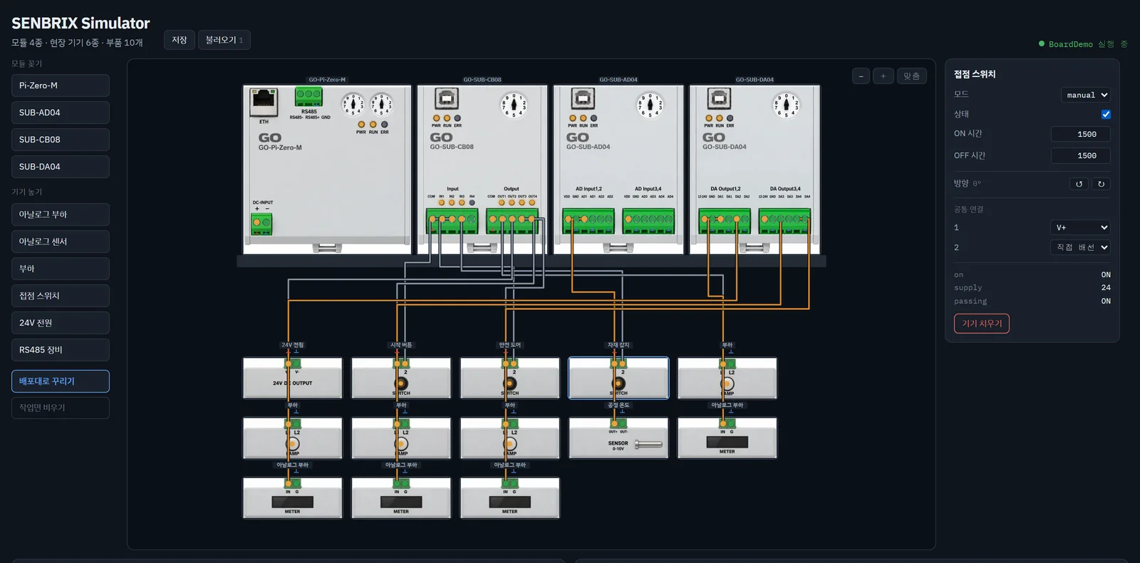
Start button, safety door and material sensor switched on one after another. supply 24 in the inspector on the right is the voltage actually present on one side of the switch, which is why passing is ON. The outputs the PLC program answered with are lit on the lamps.
Wiring by hand
The deploy does it all, but sometimes you want to build it yourself. Pick modules and devices from the list on the left and double-click terminals to connect them. Pairs that cannot be connected are refused.
As wires pile up they cross each other and run over parts. So wires can be grabbed and moved. One wire is three segments.
| Segment grabbed | Movement |
|---|---|
| The vertical runs at each end | Step sideways |
| The horizontal run in the middle | Change lane up or down |
A vertical run can only go sideways and a horizontal run only up or down. The cursor tells you which before you press. The two vertical runs move independently — when they shared one value, clearing an overlap on one side dragged the other along.
The bench zooms with the wheel and pans by dragging the background. It used to shrink everything to fit the window width, which meant the more devices you placed the smaller it all got. A screen built for wiring that got worse the more you wired.
Rotate to place, save by name
Adding RS485 devices needed one more wiring lane. That device naturally sits above the main module, but the wiring lanes had only been laid below the rail, so a device placed above got a strange route that dipped down and came back up. A lane was added above, and while at it, modules and devices became rotatable. Which way a terminal faces decides which way its wire leaves, so you gain the freedom to change the layout.
Rotate, and the labels flipped along. Seeing a device’s name upside down after a 180° turn, only the text was set upright again. You do not find this out until you rotate.
And a bench you have laid out is saved under a name and loaded later. Save and load sit next to the title. No more rebuilding the bench for every project.
RS485 devices are virtual too
This took the longest in this release.
What a PLC talks to over RS485 in the field is usually an inverter. But an inverter is not something you put on a desk to test. So the simulator has virtual RS485 devices. Connect one to the main module’s RS485 terminals, and the program’s Modbus RTU master communicates exactly as it would with the real device.
The principle is the same here. The communication master is the code inside the real runtime. The master believes it has opened a serial port, and on the other end of that port sits a virtual device placed on screen. On the controller side, as with the CAN slot, only the serial port slot was replaced.
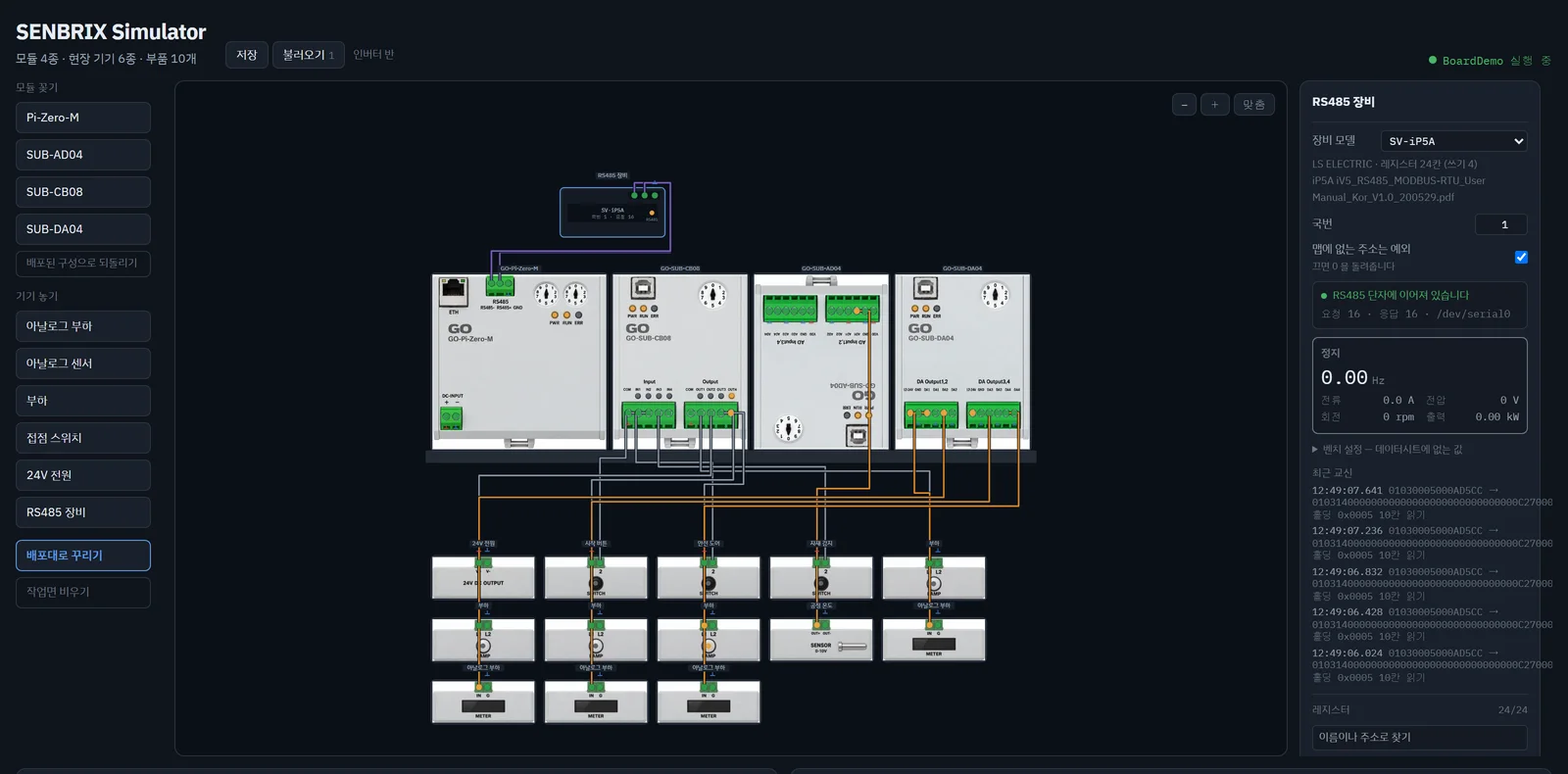
The inverter sits above the main module with its A and B wires on the RS485 terminal block. The program’s Modbus RTU master reads ten holding registers from 0x0005 every 200 ms, and each request and response frame stacks up in the inspector on the right. No run command has been given yet, so it shows 0.00 Hz, stopped.
Exactly means this. Each manufacturer’s communication register map was transcribed from the manual, so reading an address that exists returns its value and reading one that does not returns an exception, as the real device would. And when it receives a command it moves like that device. Give it a frequency reference and it ramps up over the acceleration time; the status word’s bits rise in the order the manual describes; when it trips, it stays tripped until a reset command. Stop polling and the motor keeps turning. Because the real one does.
Six register maps ship in this first release.
| Device | Reacts to commands |
|---|---|
| LS ELECTRIC SV-iP5A | Yes |
| LS ELECTRIC SV-iV5 | Yes |
| YASKAWA GA500 | Yes |
| SIEMENS SINAMICS V20 | Yes |
| Mitsubishi inverter (QPLC communication example) | Yes |
| ADT iMaster-U1 | Register read/write only |
We fell over twice here.
First. The register tables were pulled from the manual PDFs into a spreadsheet and converted, and when checked against the manuals later, more than half the addresses were missing. On another model the scale factors had slipped into the unit column. Tables breaking across page boundaries. In the end the PDFs were opened and transcribed by hand, and which section of which manual each device came from is recorded alongside. When something turns out wrong later, you need to know where to look.
Second. After transcribing five models it became clear that every manufacturer shapes the run command differently. Separate forward and reverse bits; one run bit with a separate direction bit; enables that are active low; a command written to the same address the status is read from. All four shapes had to work inside the simulator, so the plan of “do one inverter and copy the rest” was dropped as soon as the first one was done.
Write your own device’s register map as JSON, drop it in the Devices/ folder, and it joins the list. Same as the field devices.
The product artwork was redone
This is where one big step was taken back.
The module pictures had been cropped from studio renders made earlier. All of them were high-angle. Great as product photos, but laid flat on screen with wiring attached, every connector, rotary switch and terminal block looked tilted. You could tell they were cut out.
Keeping the same design, the viewpoint was remade as an orthographic front view with no perspective. No top or side of the case visible, dials and screw heads as undistorted circles, the DIN clip at the bottom not cut off.
One thing was ordered that way on purpose. Every indicator LED off. An unlit lens is the OFF state, and when the simulator lights it up on top, it looks like a real indicator coming on. Bake a state into the picture and it will disagree with reality — same reason as the labels.
The five field devices follow the same rule. 24 V supply, contact switch, lamp, analog sensor, meter. Each has a green screw terminal block along the top edge with terminal names printed large. They look like products, not gray boxes.
Terminal and indicator coordinates were not eyeballed. The screw holes inside the green terminal block and the round lenses on the housing were read straight from the picture, so the on-screen terminal sits exactly on the screw in the photo.
What is done so far
- First public release 0.1.0, and 0.1.1 — which fixes device labels being hidden behind wires — is current. It is on the Release.Senbrix release page as
Senbrix-sim-0.1.1-win.zip. One zip, 66 MB; unzip it and there is one EXE. Double-click, no .NET install - It carries runtime 0.9.2. The simulator does not reimplement the runtime; it carries that exact version, so every release states which runtime is inside. As with the Raspberry Pi, a deploy is refused if the editor is newer
- 10 parts — 4 modules, 6 field devices. 6 RS485 device register maps. Drop in one JSON file and there is one more
- 251 tests. The frame-format tests are checked against the real board drivers, and RS485 is checked by passing through the real Modbus RTU master — write it down among ourselves and the tests keep passing when a driver changes while only the simulator quietly drifts
- On launch only the modules are on display; no devices, no wiring. Deploy and they appear. An empty rail cannot even tell you what is in the product family, so the catalog is stood up only while nothing is deployed
What is not yet
The analog input module’s transfer characteristic is still an assumption. It is the curve from terminal voltage to the board’s raw value, and the resistor that sets the input range is not yet final. For now the assumed curve is used and the screen says “assumed curve”. Once it is settled, it must be replaced with measurements.
Load current through a contact is not in the model yet either. The lamp lights correctly, but that current is not deducted from the supply’s capacity.
Inverters, too, follow only what their manuals specify. Physical quantities the manual does not define — the acceleration curve, the current — are filled in with values typical of an inverter. Enough to verify a program’s communication procedure and command sequence; not a stand-in for a specific model’s fine characteristics. The iMaster-U1 has no communication command area in either of its documents, so it ships as a register map with no behavior.
Still, what we wanted works. Press deploy in the editor and modules appear on screen, sensors and switches are placed, wires are drawn, and flip a switch and the program reacts. And now give the inverter a frequency and the inverter on screen ramps up.
On a desk with no Raspberry Pi, no IO modules and no inverter, you can deploy, wire and run. A program that ran correctly in the simulator runs correctly on the Raspberry Pi. It is the same code. That is the one promise kept while building this.
🔧 GO Modular IO series: Part 1 — the system · Part 2 — the main module · Part 3 — the three sub-modules · Part 4 — specs and expansion · Part 5 — the simulator
Contact
- Email: [email protected]
- Instagram: https://www.instagram.com/going.sen/
- Website: https://intosen.com/kr/consult/
Comments
Enter a nickname to leave a comment, or sign in with Google or GitHub.